Basics on GNSS Meteorology

”GNSS-Meteorology ….It involves the use of GNSS satellites to obtain atmospheric profiles of Temperature pressure and water vapour/humidity…”

Global Navigation Satellite Systems (GNSS)

TRANSIT, was the first operational satellite navigation system. The system was developed to provide accurate location information to ballistic missile submarines. The system was rolled out for military use in January 1964 and subsequently to civilian users in July 1967. The system, using a constellation of five polar orbiting satellites in low Earth orbit (1075km) was comprised of 2 carrier frequencies (150 and 400MHz) which could be used to provide an hourly positioning estimate with an accuracy of between 200 and 400m. However, at early of 1990 the Global Positioning System (GPS) achieved operational capability that continuous 3 dimensional positioning and timing information became widely available allowing positioning accuracy down to the sub decimetre level. The basic principle of GPS is that coded signals are transmitted by at least four satellites for the 3 dimensional positions, plus the time element, to be determined. More information on the technique is given in the section below focusing on GPS basics.

GPS Basics

GPS is the shortened form of NAVSTAR GPS. This is an acronym for NAVigation System with Time And Ranging Global Positioning System. GPS is a satellite-based system that uses a constellation of 24 satellites orbiting the earth at approximately 20200km every 12 hours to give a user an accurate position. There must be at least 24 satellites operational to ensure any point on the Earth’s surface can “see” at least 4 satellites at any one time. Each GPS satellite has several very accurate atomic clocks on board. The clocks operate at a fundamental frequency of 10.23MHz. This is used to generate the signals that are broadcast from the satellite. The satellites transmit coded signals and other information (orbital elements/parameters, satellite clock errors etc.) to the user. The ground segment consists of a master control station in Colorado, USA as well as a number of global (>10) monitoring stations which are responsible for generating the satellite information such as orbits and clock errors. The basic principle to estimate Position Velocity and Time is the triangulation. At least four satellites are needed to compute the four unknowns, the three position coordinates and one clock error. The user segment performs two basic measurements of the GNSS signals. It compares the code that is received with a locally generated copy in order to compute the transmission delay between the satellite and the receiver. This measurement is called Pseudorange. Pseudorange use four or more satellites to determine the position of the user after the position of the GPS satellites has been obtained using the ephemerides from the navigation message. The second and more precise method is to obtain the difference in phase between the received carrier signal and a receiver-generated signal at the same frequency. This measurement is known as the carrier phase observable and it can reach millimeter precision, but it lacks the accuracy of the pseudorange because the phase when the tracking is started can only be known with an ambiguity of an unknown number of times the carrier wavelength.

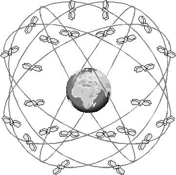
Representation of the GPS Satellite constellation

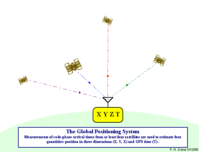
Illustration of GPS 3D positioning

GLONASS Basics

GLONASS is the Russian global satellite navigation system, providing real time position and velocity determination for military and civilian users. GLONASS satellite constellation consists (today) of 26 space vehicles, evenly distributed in three orbital planes. Satellites operate in circular orbits at altitudes of 19,100 km. This configuration permits uninterrupted global coverage of the Earth’s surface and terrestrial space by the navigation field. Glonass-M space vehicles with operational lifetimes of seven years transmit navigation signals in L1 and L2 frequency bands. The GLONASS satellites' designs have undergone several upgrades, with the latest version being GLONASS-K2, scheduled to enter service within 2018. The geometry repeats about once every 8 days. The orbit period of each satellite is approximately 8/17 of a sidereal day such that, after eight sidereal days, the GLONASS satellites have completed exactly 17 orbital revolutions. A sidereal day is the rotation period of the Earth relative to the equinox and is equal to one calendar day (the mean solar day) minus approximately four minutes.

• Because each orbital plane contains eight equally spaced satellites, one of the satellites will be at the same spot in the sky at the same sidereal time each day.

• The satellites are placed into nominally circular orbits with target inclinations of 64.8 degrees and an orbital height of about 19,140 km, which is about 1,050 km lower than GPS satellites.

• Some of the GLONASS transmissions initially caused interference to radio astronomers and mobile communication service providers. The Russians consequently agreed to reduce the number of frequencies used by the satellites and to gradually change the L1 frequencies in the future to 1598.0625 – 1605.375 MHz. Eventually the system will only use 12 primary frequency channels (plus two additional channels for testing purposes).

The GLONASS satellite signal identifies the satellite and provides:

• position, velocity and acceleration vectors at a reference epoch to compute satellite locations
• synchronization bits, data age and satellite health
• offset of GLONASS time from UTC (RU)
• almanacs of all other GLONASS satellites

GLONASS Time and Datum

GLONASS time is based on an atomic time scale similar to GPS. This time scale is UTC as maintained by Russia (UTC (SU)). A datum is a set of parameters (translations, rotations, and scale) used to establish the position of a reference ellipsoid with respect to points on the Earth’s crust. If not set, the receiver’s factory default value is the World Geodetic System 1984 (WGS84). GLONASS information is referenced to the Parametri Zemli 1990 (PZ-90, or in English translation, Parameters of the Earth 1990, PE-90) geodetic datum, and GLONASS coordinates are reconciled in the receiver through a position filter and output to WGS84. More infos about GLONASS status are available at https://www.glonass-iac.ru/en/GLONASS/

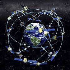
Representation of the GLONASS Satellite constellation (source:internet)

GNSS User Errors

GNSS User Equivalent Errors (USER) is defined as the errors in 3D position and time computation due to three segments of GNSS architecture. In space segment, the source of error can be satellite clock stability, satellite perturbations or selective availability (turned off in May 2001). The control segment causes the errors like ephemeris prediction and the user segment contributes the major part due to Ionospheric delay, Tropospheric delay, multipath and receiver noise.

• Satellite and receiver clock errors
• Satellite orbit errors
• Atmospheric effects (ionosphere, troposphere)
• Multipath: signal reflected from surfaces near the receiver
• Antenna phase center
• Solar radiation pressure
• Satellite Geometry
• Relativistic Effects
• Receiver noise
• Signal Obstructions

Process of GNSS Data

We process station GNSS data using the world famous Bernese processing software. Bernese GNSS Software is a scientific, high-precision, multi-GNSS data processing software developed at the Astronomical Institute of the University of Bern (AIUB). It is, e.g., used by CODE (Center for Orbit Determination in Europe) for its international (IGS) and European (EUREF/EPN) activities. The software is in a permanent process of development and improvement. The current version the Bernese GNSS Software is "5.2", with the release date of "2018-02-28". More infos about Bernese software are available at http://www.bernese.unibe.ch/.

Zenith Tropospheric Delay Estimates using GNSS data

At it is already mentioned, Global Navigation Satellite Systems (GNSS), including the United States Global Positioning System (GPS), the Russian GLONASS (Globalnaja Nawigazionnaja Sputnikowaja Sistema), the European Galileo, and others use satellites at orbital heights of about 20200km that transmit microwave signals received by antennae at the Earth surface. Over the past 20 years, the applications of GPS technologies and nowadays GNSS have been developed in many different areas. One of these areas is the GPS meteorology, which means the use of GPS data for climate monitoring through analysis of several atmospheric parameters, such as the Precipitable Water (PW). The principle is that the atmospheric gases, including water vapor in atmosphere cause an additional delay (range error) in GNSS observations as the broadcast signals from satellites travel through the neutral atmosphere to gps receivers. This delay can be modeled and estimated by a parameter called total Zenith Tropospheric Delay (ZTD). Therefore ZTD is an important parameter of the atmosphere, which reflects the weather and climate processes, variations and atmospheric motions. Ground-based GNSS tropospheric delay sensing relies on a network of geodetic-quality dual-frequency receivers at known locations, precise orbit models, and accurate models relating temperature and moisture content in the atmosphere. High-precision software like Bernese must be used to ensure that all other error sources have been eliminated. Several research projects using continuous observations from GNSS permanent networks stations were initiated in Europe and overseas for mapping and predict the state of the atmosphere and as a consequence the climate changes. One of the standard outputs from a number of geodetic GPS processing (research oriented) software is ZTD based on phase measurements from a network of ground based GPS receivers. In GPS meteorology it is useful to reduce the term of ZTD into its constituent parts, Zenith Hydrostatic Delay (ZHD) and Zenith Wet Delay (ZWD). ZHD is responsible for the vast majority of the ZTD delay (typically around 90%) and is easily modelled if surface pressures are known. It is the ZWD which is of interest to meteorology as it is this component which is related to humidity and can change rapidly both spatially and temporally. If we assume that the dry and wet components of equation 2.7 behave as ideal gases, Zd and Zw are equal to 1 (Bevis et al., 1992) and can therefore be eliminated. Such that, we separate the pressure into its dry and wet partial pressures.

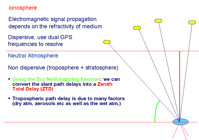
Schematic of Satellite signal path through atmosphere

The Near Real Time GNSS delay data contain information about the amount of water vapour above the GNSS sites. Water vapour plays a key role in some of the most important weather phenomena: It is obviously related to precipitation, but also provides about half the energy to the atmosphere (via latent heat release), contributing to atmospheric dynamics, and it is the dominant greenhouse gas. There is a big lack of humidity observations in the meteorological observing system, usage of ground based GNSS data is one means by which to improve on this.

Estimation of Precipitable Water values using GNSS data

Precipitable water (PW) is the depth of water that would result if all atmospheric water vapor in a vertical column of air condensed to liquid while the IWV is the Integrated Water Vapour content of the atmosphere (IWV). The continuous record of PW estimates and meteorological variables is highly recommended for further studies on the behavior of the atmospheric water vapor and its contribution to the climate monitoring.

Estimated zenith wet delays (ZWD) by GPS (ZWD = ZTD –ZHD) can be converted to PW using the formula:

The Q factor is expressed as

Where ρ is the density of liquid water, R0 is the universal gas constant, MW is the molar mass of water vapor and Tm is the weighted mean temperature of the atmosphere in [K]. The physical constants k’2 and k3 are taken from Davis et al. (1985).

Where,

Finally the Q factor is given by,

Concerning the parameter Tm, Bevis et al., (1992) suggested that it can be estimated from the surface temperature Ts because of the strong correlation between the two variables. In our study the parameter Tm was estimated Zaccording to the formula by Mendes et al. (2000) which holds for mid-latitudes.

where, Ts: surface temperature in [Kelvin] and Tm: mean temperature of the atmosphere in [Kelvin]. Introducing a combination of the above equations, then we finally get that:

Combine the equations and applying all the polynomials calculations, we finally get that PW equals to (Katsougiannopoulos, et. al., 2015):

The above formula was used in our study. The ZWD is given in [mm] and the surface temperature Ts in [K]. This equation is a useful formula to calculate the PW (in mm) from ZWD values, introducing only the surface temperature Ts. This formula is suitable for mid- latitudes like in case of Hellenic territory.

IMPORTANT NOTICE

All of the hourly produced MAPS based on the GNSS_Meteorology theory can be freely downloaded by the following FTP address: 155.207.25.81/usbshare1/BeRTISS_MAPS. (Input FTP info[ ] UserName:user and password:anonymous)

Other GNSS systems

Galileo is the global navigation satellite system(GNSS) that is currently being created by the European Union (EU) through the European Space Agency (ESA). The fully deployed Galileo system will consist of 24 operational satellites plus six in-orbit spares, positioned in three circular Medium Earth Orbit (MEO) planes at almost 23 000 km altitude above the Earth, and at an inclination of of 56 degrees to the equator. https://www.esa.int/Our_Activities/Navigation/Galileo/What_is_Galileo

BeiDou Navigation Satellite System (BDS) is a Chinese satellite navigation system. In 1993, China decided to implement an independent navigation system called BEIDOU. The name BEIDOU denotes the seven-star constellation also known as Ursa Major, Great Cart, or Big Dipper. This constellation has been used for centuries to identify the star Polaris, which indicates the north direction on the northern hemisphere. In its first development step, BEIDOU was aimed to provide service to China and parts of neighbouring countries by 2008. The system architecture is similar to the other global systems. According to the Radio Regulatory Department (2006), the BEIDOU-2 satellite constellation will consist of 27 MEO satellites, 5 satellites in geostationary orbit (GEO), and 3 more satellites in geosynchronous orbit. The 27 MEO satellites will have an average satellite altitude of 21500 km. BEIDOU BDS-2 (earlier referred to as COMPASS) comprises a total of 15 launched satellites out of which 13 were fully operational in 2015. In mid-2015, China started the build-up of the 3rd generation BEIDOU system (BDS-3) which will shall offer a fully global navigation service by 2020. So far, five BDS-3S in-orbit validation satellites have been launched. In the absence of official space vehicle numbers (SVNs), preliminary numbers for the above satellites have been assigned for use within the MGEX project http://mgex.igs.org/ based on the launch sequence of the respective spacecraft. PRN numbers have been associated with the individual satellites based on comparison of transmitted ranging codes with code sequences in the BEIDOU Interface Control Document (ICD). The latest version of the Open Service Signal ICD (BEIDOU Navigation Satellite System Signal In Space Interface Control Document - Open Service Signal (Version 2.1)) covers the B1I and B2I signals and has been released in November 2016. A comprehensive collection of technical information with associated references for the BEIDOU-2 satellites can be obtained at the CNSS page of ESA's eo Portal https://directory.eoportal.org/web/eoportal/satellite-missions/.

************************************************************************

All the team members of GNSS_QC are currently working on the estimation of Tropospheric products using Multi GNSS data in order to improve the role of GNSS systems in some of the most important weather phenomena.

************************************************************************

General References (also used on this Project):

Askne J., and Nordius H. (1987). Estimation of tropospheric delay for microwaves from surface weather data, Radio Science, Vol 22(3): 379-386.

Böhm J., Werl B., and Schuh H. (2006). Troposphere mapping functions for GPS and very long baseline interferometry from European Centre for Medium-Range Weather Forecasts operational analysis data, J. Geophys. Res., 111, B02406, doi:10.1029/2005JB003629.

Boehm J., G. Moeller, M. Schindelegger, G. Pain, R. Weber. (2015). Development of an improved blind model for slant delays in the troposphere (GPT2w), GPS Solutions, 2014. Doi: 10.1007/s10291-014-0403-7.

Brenot H., V. Ducrocq, A. Walpersdorf, C. Champollion, and O. Caumont (2006). GPS zenith delay sensitivity evaluated from high-resolution numerical weather prediction simulations of the 8–9 September 2002 flash flood over southeastern France, J. Geophys. Res., 111, D15105, doi:10.1029/2004JD005726.

Caissy M., Agrotis, L., Weber G., Hernandez-Pajares, M., and Hugentobler, U. (2012). INNOVATION-Coming Soon-The International GNSS Real-Time Service, GPS World, 23, 52–58.

Dach R., Lutz S., Walser P., and Fridez, P. (2015). User manual of the Bernese GNSS Software, Version 5.2. University of Bern, Bern Open Publishing, doi:10.7892/boris.72297.

Davis J.L, T.A. Herring I.I. Shapiro A.E.E. Rogers and G. Elgered. (1985). Geodesy by Radio Interferometry: Effects of Atmospheric Modeling Errors on Estimates of Baseline Length, Radio Science, Vol. 20, No. 6, pp. 1593-1607, 1985.

Davis J.L., Elgered G., Niell A.E., and Kuehn C.E. (1993). Ground based Measurements of Gradients in the “Wet” Radio Refractivity of air. Radio Science, 28, 1003–1018.

Douša J. (2001). Towards an Operational Near-real Time Precipitable Water Vapor Estimation, Physics and Chemistry of the Earth Pt. A, 26, 189–194. doi:10.1016/S1464-1895(01)00045-X.

Douša J. (2001). The Impact of Ultra-Rapid Orbits on Precipitable Water Vapor Estimation using Ground GPS Network, Physics and Chemistry of the Earth, 26(6-8):393-398.

Douša J. (2004). Evaluation of tropospheric parameters estimated in various routine analysis, Physics and Chemistry of the Earth, 29(2-3):167-175.

Douša J. and Bennitt G.V. (2013). Estimation and evaluation of hourly updated global GPS Zenith Total Delays over ten months, GPS Solutions, 17, 453–464, doi:10.1007/s10291-012-0291-7.

Fotiou A. and Pikridas C. (2012). GPS & Geodetic Applications.ISBN:978960456346-3, Eds: Ziti-Thessaloniki, Greece.

Gendt G., Dick G., Reigber,C., Tomassini M, Liu, Y., and Ramatschi M. (2004). Near Real Time GPS Water Vapor Monitoring for Numerical Weather Prediction in Germany, J. Meteorol. Soc. Japan, 82, 361–370.

Guerova G, Jones J, Douša, J, Dick G, de Haan S, Pottiaux E, Bock O, Pacione R, Elgered G, Vedel H, Bender M. (2016). Review of the state of the art and future prospects of the ground-based GNSS meteorology in Europe, Atmos. Meas. Tech., 9, 5385-5406, doi:10.5194/amt-9-5385-2016.

Hatanaka Y. (2008): A Compression Format and Tools for GNSS Observation Data, Bulletin of the Geographical Survey Institute, 55, 21-30, available at http://www.gsi.go.jp/ENGLISH/Bulletin55.html.

Ifadis I. M. (1993). Space to Earth Techniques: Some Considerations on the Wet Delay Parameters, Survey Review, pp. 32, 249.

Karabatic A., Weber R., Haiden T., Near real-time estimation of tropospheric water vapour content from ground based GNSS data and its potential contribution to weather now-casting in Austria (2010). in: Advances in Space Research, 47, 10, pp. 1691-1703, doi:10.1016/j.asr.2010.10.028.

Katsougiannopoulos S., (2008). Study of tropospheric effect on GNSS signals. Application to the European area. PhD Thesis, Department of Geodesy and Surveying, Faculty of Enginnering, Aristotle University of Thessaloniki, Greece.

Nakamura S. (1991). Applied Numerical Methods with Software, Prentice-Hall Inc.

Niell A. E. (1996). Global mapping functions for the atmosphere delay at radio wavelengths, J. Geophys. Res., 101, 3227–3246, doi: 10.1029/95JB03048.

Ning T., Wang, J., Elgered G., Dick G., Wickert J., Bradke M., and Sommer, M. (2016). The uncertainty of the atmospheric integrated water vapour estimated from GNSS observations, Atmos. Meas. Tech.., 9, 79-92, doi:10.5194/amt-9-79-2016.

Václavovic P. and Douša, J. (2015). Backward smoothing for precise GNSS applications, Advances in Space Research, 56(8):627-1634, doi:10.1016/j.asr.2015.07.020.

Walpersdorf A., Calais E., Haase J., Eymard L., Desbois M., and Vedel, H. (2001). Atmospheric Gradients Estimated by GPS Compared to a High Resolution Numerical Weather Prediction (NWP) Model, Phys. Chem. Earth, 147–152.

Pikridas C., (2014). Monitoring climate changes on small scale networks using ground based GPS and meteorological data. Journal of Planetary Geodesy-Artificial Satellites, vol. 49, No. 3. Walter De Gruyter.

Saastamoinen, J. (1972). Atmospheric correction for the troposphere and stratosphere in radio ranging of satellites. The use of artificial satellites for geodesy, Geophys. Monogr. Ser. 15, Amer. Geophys. Union, pp. 274-251, 1972.

Thomas Nischan (2016): GFZRNX - RINEX GNSS Data Conversion and Manipulation Toolbox (Version 1.05). GFZ Data Services. http://doi.org/10.5880/GFZ.1.1.2016.002.

TEQC: The Multi-Purpose Toolkit for GPS/GLONASS Data, L. H. Estey and C. M. Meertens, GPS Solutions (pub. by John Wiley & Sons), Vol. 3, No. 1, pp. 42-49, doi:10.1007/PL00012778, 1999.

Teunissen P., A. Kleusberg, Y. Bock, G. Beutler, R. Weber, R. B. Langley, H. van der Marel, G. Blewitt, C. C. Gload and O. L. Colombo (1998) GPS for Geodesy, Springer, 2nd Edition.

Tregoning P. and T. van Dam (2005). Atmospheric pressure loading corrections applied to GPS data at the observation level. Geophysical Research Letters, 32(22), 1–4. http://doi.org/10.1029/2005GL024104.

Zus F., Dick, G., Heise S., and Wickert, J. (2015). A forward operator and its adjoint for GPS slant total delays, Radio Sci., 50, 393–405.

Zumberge J.F.; Heflin, M.B.; Jefferson, D.C.; Watkins, M.M.; Webb, F.H. (1997) Precise Point Positioning for the efficient and robust analysis of GPS data from large networks, J. Geophys. Res., 102, 5005–5017. doi:10.1029/96JB03860.

Wessel P., W. H. F. Smith, R. Scharroo, J. Luis and F. Wobbe (2013). Generic Mapping Tools: Improved Version Released. Eos, Transactions American Geophysical Union, 94(45), 409–410. http://doi.org/10.1002/2013EO450001.